Hands-on Neural Networks
In this section we will build a simple neural network, train it and validate it on a sample test data. For this excercise we will use a popular dataset from Keras, known as the MNIST (Modified National Institute of Standards and Technology) dataset. This dataset is collection of around 70,000 images of size 28X28 pixels of handwritten digits from 0 to 9 and our goal is to accurately identify the digits by creating a Neural Network.
By the end of this excercise students will be able to:
Import the Keras MNIST dataset.
Pre-process images so they are suitable to be fed to the neural network.
Apply data preprocessing for converting output labels to one-hot encoded variables.
Build a sequential model neural network.
Evaluate the model’s performance on test data.
Add more layers to the neural network and evaluate if the model’s performance improved or degraded, leveraging the same test data.
Step 1: Importing required libraries and data
We know that the mnist dataset is available in keras so we will first import keras and then import the dataset.
MNIST has a training dataset of 60,000, 28x28 grayscale images of handwritten digits 0-9, along with a test data of 10,000 grayscale images of size 28x28 pixels (0-9 digits).
import keras
from keras.datasets import mnist
We will load the training and test data directly, as below
(X_train, y_train), (X_test, y_test) = mnist.load_data()
This returns a tuple of numpy arrays: (X_train, y_train), (X_test, y_test).
# Shape of training data. X_train contains train images and y_train contains output labels for train images
print(X_train.shape)
print(y_train.shape)

# Shape of test data. X_test contains test images and y_test contains output labels for test images
print(X_test.shape)
print(y_test.shape)
X_train is 2-D array of 60000 images of size 28 x 28 pixels.
y_train is a 1D array with 60000 labels
Step 2: Image Pre-processing
A grayscale image is an image where each pixel is represented by a single scalar value
indicating the brightness or intensity of that pixel.
Color images have three channels (e.g., red, green, and blue) whereas grayscale images have only one channel.
In a grayscale image, the intensity value of each pixel typically ranges from 0 to 255, where 0
represents black (no intensity) and 255 represents white (maximum intensity).
Grayscale images are commonly used in various image processing and computer vision tasks, including image analysis, feature extraction, and machine learning. They are simpler to work with as compared to color images, as they have only one channel, making them computationally less expensive to process. Additionally, for certain applications where color information is not necessary, grayscale images can provide sufficient information for analysis.
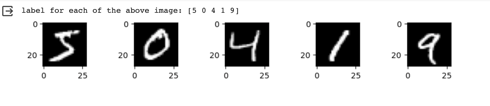
Lets look at few sample images from the dataset along with their labels.
import matplotlib.pyplot as plt
plt.figure(figsize=(10, 1))
for i in range(5):
    # Subplot will plot 5 images in 1 row.
    plt.subplot(1, 5, i+1)
    plt.imshow(X_train[i], cmap="gray")
print('label for each of the above image: %s' % (y_train[0:5]))
The first parameter of subplot represents the number of rows, the second represents the number of
columns and the third represents the subplot index. Subplot indices start from 1, so i+1 ensures
that the subplot position starts from 1 and increases by 1 in each iteration.
Each image has a total of 784 pixels representing intensities between 0-255. Each of these pixel values
is treated as an independent feature of the images. So the total number of input dimensions/features of the
images is equal to 784. But the image provided to us is 2D array of size 28x28. We will have to reshape/flatten it
to generate a 1D vector of size 784 (28*28) so it can be fed to the very first dense layer of the neural network.
We will use the reshape method to transform the array to desired dimension.
# Flatten the images
image_vector_size = 28*28
X_train = X_train.reshape(X_train.shape[0], image_vector_size)
X_test = X_test.reshape(X_test.shape[0], image_vector_size)
reshape is a numpy array method that changes the shape of the given array without changing the
data. By reshaping X_train with the specified shape (i.e., image_vector_size),
each image in the training dataset is flattened into a one-dimensional array of size image_vector_size.
Next, we normalize the image pixels, which is a common preprocessing step machine learning tasks, particularly in computer vision, where it helps improve the convergence of models during training. Normalization typically involves scaling the pixel values to be within a specific range, such as [0, 1]
You can either use Keras.preprocessing API to rescale or simply divide the number of pixels by 255. For this example, we are adopting the later approach
X_train_normalized = X_train / 255.0
X_test_normalized = X_test / 255.0
Step 3: Data pre-processing on output column.
We see that the dependent or target variable (y_train) that we want to predict is a
categorical variable and holds labels 0 to 9. We have previously seen that we can one-hot encode
categorical variables. Here we use utility function from keras.util to convert to
one-hot encoding using the to_categorical method.
from tensorflow.keras.utils import to_categorical

# Convert to "one-hot" vectors using the to_categorical function
num_classes = 10
y_train_cat = to_categorical(y_train, num_classes)
Question: Can you guess what will be y_train_cat[0]?
Step 4: Building a sequential model neural network
Let’s now create a neural network. We will create a neural network one input layer, one hidden layer and one output layer and check its prediction accuracy on the test data.
We will need to import Sequential and Dense from Keras.
# Importing libraries needed for creating neural network,
from tensorflow.keras import Sequential
from tensorflow.keras.layers import Dense

image_size=28*28

# create model
model = Sequential()
# input layer
model.add(Dense(784, activation='relu',input_shape=(image_size,)))

# Hidden layer
model.add(Dense(128, activation='relu'))

# Softmax activation function is selected for multiclass classification
model.add(Dense(10, activation='softmax'))
Here you must havee noticed that we used softmax activation function.
The softmax activation function is commonly used in the output layer of a neural network, especially in multiclass classification problems.
It normalizes the output of a neural network into a probability distribution over multiple classes, ensuring that the sum of the probabilities of all classes is equal to 1.
Let’s compile and fit the model
model.compile(optimizer='adam', loss='categorical_crossentropy', metrics=['accuracy'])
model.fit(X_train_normalized, y_train_cat, validation_split=0.2, epochs=5, batch_size=128, verbose=2)
Here we use the same Adam optimizer, binary cross entropy and accuracy as metrics, that we had used before. validation_split parameter specifies the fraction of the training data to use for validation. In this case, 20% of the training data will be used for validation during training, and the remaining 80% will be used for actual training. epochs=5: The number of epochs (iterations over the entire training dataset) to train the model. In this case, the model will be trained for 5 epochs.
Epoch 1/5
375/375 - 3s - loss: 0.0598 - accuracy: 0.9095 - val_loss: 0.0272 - val_accuracy: 0.9594 - 3s/epoch - 8ms/step
Epoch 2/5
375/375 - 2s - loss: 0.0202 - accuracy: 0.9693 - val_loss: 0.0188 - val_accuracy: 0.9708 - 2s/epoch - 5ms/step
Epoch 3/5
375/375 - 2s - loss: 0.0129 - accuracy: 0.9816 - val_loss: 0.0150 - val_accuracy: 0.9766 - 2s/epoch - 5ms/step
Epoch 4/5
375/375 - 2s - loss: 0.0089 - accuracy: 0.9879 - val_loss: 0.0149 - val_accuracy: 0.9763 - 2s/epoch - 5ms/step
Epoch 5/5
375/375 - 2s - loss: 0.0061 - accuracy: 0.9921 - val_loss: 0.0154 - val_accuracy: 0.9776 - 2s/epoch - 5ms/step
375/375: Indicates that the training process has completed 375 batches out of a total of 375 batches. This suggests that the entire training dataset has been processed in 375 batches during the training process.
Time in seconds indicates that the training process took approximately 2/3 seconds to complete that epoch.
loss indicates the value of the loss function (typically categorical cross-entropy loss for classification tasks) computed on the training dataset.
accuracy Represents the accuracy of the model on the training dataset. The accuracy value of approximately 0.99 indicates that the model correctly predicted 98% of the training samples.
val_loss Represents the value of the loss function computed on the validation dataset.
val_accuracy Represents the accuracy of the model on the validation dataset. The validation accuracy value of approximately 0.98.
5ms/step This indicates the average time taken per training step (one forward and backward pass through a single batch) during training.
We can next print the model summary. It shows how many trainable parameters are in the Model
model.summary()

Here the total parameters and number of trainable parameters is same which is 717210. It is calculated as follows:
- Total weights from previous layer + Total bias for each neuron in current layer
784*784 + 784 = 615440
Optional: In order to see the bias and weights at each epoch we can use the helper function below
from tensorflow.keras.callbacks import LambdaCallback
 # Define a callback function to print weights and biases at the end of each epoch
def print_weights_and_biases(epoch, logs):
    if epoch % 1 == 0:  # Print every epoch
        print(f"\nWeights and Biases at the end of Epoch {epoch}:")
        for layer in model.layers:
            print(f"Layer: {layer.name}")
            weights, biases = layer.get_weights()
            print(f"Weights:\n{weights}")
            print(f"Biases:\n{biases}")

# Create a LambdaCallback to call the print_weights_and_biases function
print_weights_callback = LambdaCallback(on_epoch_end=print_weights_and_biases)
When we fit the model, we will specify the callback parameter
model.fit(X_train_normalized, y_train_cat, validation_split=0.2, epochs=5, batch_size=128, verbose=2,callbacks=[print_weights_callback])
This will print all the weights and biases in each epoch.
Once we fit the model, next important step is predicting on the test data.
Step 5: Evaluate model’s performance on test data
# predicting the model on test data
y_pred=model.predict(X_test_normalized)
We can see the predictions by printing the y_pred values.
y_pred[0]
output
array([1.9272175e-17, 3.0873656e-17, 2.3461717e-19, 1.8416815e-16,
   4.0177441e-22, 5.5508965e-21, 1.2490869e-21, 9.9999994e-01,
   1.5065967e-18, 1.9806202e-16], dtype=float32)
As you can see the output values are probabilities so we will try to get the output class from these probablities by getting the maximum value
import numpy as np
y_pred_final=[]
for i in y_pred:
    y_pred_final.append(np.argmax(i))
Visualizing the model’s prediction accuracy with confusion matrix
With confusion matrix we can see how many correct vs incorrect predictions were made using the model above.
from sklearn.metrics import confusion_matrix
import seaborn as sns

cm=confusion_matrix(y_test,y_pred_final)

plt.figure(figsize=(10,7))
sns.heatmap(cm,annot=True,fmt='d')
plt.xlabel('Predicted')
plt.ylabel('Truth')
plt.show()
Output of the above confusion matrix is as follows
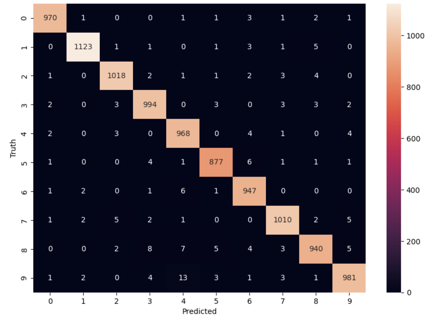
The numbers highlighted accross the diagonals are correct predictions. While the numbers in black squares are number of incorrect predictions.
Let’s also print the accuracy of this model using code below
from sklearn.metrics import classification_report
print(classification_report(y_test,y_pred_final))
As you can see the accuracy of the above model is 98%. 98% of the times this model predicted with correct label on the test data.
Class Exercise:
Let’s now repeat the hands-on part for MNIST Fashion dataset. MNIST Fashion dataset has 10 categories for apparel and accessories. Our goal is to accurately classify the images in test dataset by creating the ANN model
#0 T-shirt/top
#1 Trouser
#2 Pullover
#3 Dress
#4 Coat
#5 Sandal
#6 Shirt
#7 Sneaker
#8 Bag
#9 Ankle boot
In Step1: Loading the data, source of dataset will change to:
 # Loading the data
from tensorflow.keras.datasets import fashion_mnist
(X_train, y_train), (X_test, y_test) = fashion_mnist.load_data()
From Step 1, you may check the shape of X_train, y_train. Run through Steps 2 to 5.
Questions: - How confident are you about the model? - Does the validation accuracy improve if you run for more number of epochs or does adding more hidden layers help?