Introduction to Pandas
In this module, we will introduce the Python library pandas for working with the datsets
and manipulating them [1]. After going through this module, students should be able to:
Install and import the
pandaspackage into a Python program.Understand the primary differences between the pandas
seriesanddataframe, and when to use each.Loading data from an external file into a pandas object.
Accessing pandas
seriesanddataframeto perform various dataset manipulations.
Installing Pandas
The pandas package is available from the Python Package Index (PyPI) and can be installed on most
platforms using a Python package mananger such as pip:
[container/virtualenv]$ pip install pandas
Once installed, we can import the pandas package; it is customary to import the top level package
as pd, i.e.,
>>> import pandas as pd
Now, let’s take a look at the basic data structures supported by Pandas.
Pandas Series
A pandas Series is a one-dimensional array capable of holding data of different types (string, float, integer, objects, etc.) as well as axis labels. It can be thought of as a single column in a dataset.
We can create Series objects in different ways; for example, directly from a
numpy array or python list:
>>> a = [1, 5, 8]
>>> m = pd.Series(a)
>>> m
0    1
1    5
2    8
dtype: int64
As you can see from the output, every value in a pandas Series is labeled. If nothing is specified when constructing the Series, values are labeled staring from index 0 (i.e., the first value will have index 0, the second will have index as 1, and so on).
For instance, with the previous example, we can put:
>>> m[2]
8
This works exactly like Python lists and numpy arrays.
However, we can customize the label indexes using the index argument
while creating series.
>>> a = [1, 5, 8]
>>> m = pd.Series(a, index=["X", "Y","Z"])
>>> m
X    1
Y    5
Z    8
dtype: int64
And now we can use these custom lables to index the elements of the series; for example:
>>> m["Y"]
5
Note that if we specify custom index lables, we shouldn’t use the 0-based integer indexing to index into our series.
What happens if you try the following:
>>> m[1]
?
Custom labels for indexes provide part of the power of pandas; we can use lables to attach meaning (or “metadata”) to our data columns.
For example, say we want to create a series of back to school supplies with their cost, and we have a supplies list and a cost list as follows:
>>> supplies = ['Spiral_Notebook', 'Gel_Pens', 'Sticky_Notes', 'Laptop_Bag', 'Daily_Planner']
>>> cost_supplies_dollars = [12.81, 9.99, 5.99, 23.66, 10.99]
We can use these to create a Series as follows:
>>> supplies_cost = pd.Series(cost_supplies_dollars, index=supplies)
>>> supplies_cost
Spiral_Notebook    12.81
Gel_Pens            9.99
Sticky_Notes        5.99
Laptop_Bag         23.66
Daily_Planner      10.99
dtype: float64
We see that our series is indexed by the labels we gave for the prices. We can now access the prices using the meaningful labels, e.g.,
>>> supplies_cost['Gel_Pens']
9.99
We can even use these custom index labels in slices, but note that the slice is inclusive of both endpoints; for instance,
>>> supplies_cost["Gel_Pens":"Daily_Planner"]
Gel_Pens          9.99
Sticky_Notes      5.99
Laptop_Bag       23.66
Daily_Planner    10.99
dtype: float64
In-class Exercise:
Try accessing multiple elements of the supplies_cost series at positions 1,3 and 0.
What will be the output of following code?
>>> supplies_cost[:'Laptop_Bag']
Pandas DataFrame
The DataFrame is perhaps the most important and useful data structure in pandas. A pandas
DataFrame is similar to a 2d-array that can hold heterogeneous data and labeled axes. You can
think of a DataFrame as representing a spreadsheet or a database table with multiple columns.
Said differently, a DataFrame object is like a dictionary of Series objects.
Let’s look at some examples to make it more clear.
To begin, suppose we had information on employees at UT Austin. If we were storing this information in a spreadsheet, we might have several columns, such as:
Name
EID
Department
Location
Each employee could be thought of as a row in our spreadsheet with values for each of the columns above. For instance, we might have data on the following employees:
John Doe, E0124, Austin, ITS
Luna Lau, E0125, Houston, Student Services
Bella Tran, E1119, Austin, Accounting
Raj Kumar, E2048, Dallas, Finance
We can model these columns of data using a Pandas dataframe as follows:
>>> employees = pd.DataFrame(
    {
      'eid' :['E0124', 'E0125','E1119','E2048'],
      'name':['John Doe', 'Luna Lu', 'Bella Tran', 'Raj Kumar'],
      'location':['Austin','Houston', 'Austin', 'Dallas'],
      'department':['ITS','Student Services', 'Accounting','Finance']
    }
  )
Notice that in the above example we construct the DataFrame using a Python dictionary of lists, where each key in the dictionary represents a column in our dataset, and the corresponding list contains the values for that column.
Indexing Columns
We now have several access methods for getting at the data in our DataFrame. For example, we can access an individual column using the associated key:
>>> employees['name']
  0      John Doe
  1       Luna Lu
  2    Bella Tran
  3     Raj Kumar
  Name: name, dtype: object
This is similar to normal Python dictionary access, but notice that the output contains indexes for the employees (i.e., the rows) as well.
Indexing Rows
We can access individual rows in the data set using the iloc function, like so:
>>> employees.iloc[1]
  eid                      E0125
  name                   Luna Lu
  location               Houston
  department    Student Services
  Name: 1, dtype: object
Note
Using iloc requires the use of brackets ([]), not parenthesis (()) as with normal function
invocation.
Be aware that one cannot index into the DataFrame using an integer (row) index; it will result in an error:
>>> employees[1]
  ---------------------------------------------------------------------------
  KeyError                                  Traceback (most recent call last)
  File ~/.cache/pypoetry/virtualenvs/risd-course-KKx7_8Y0-py3.11/lib/python3.11/site-packages/pandas/core/indexes/base.py:3791, in Index.get_loc(self, key)
  3790 try:
  -> 3791     return self._engine.get_loc(casted_key)
  3792 except KeyError as err:
  . . .
This is the same error one would get if one tried to index a normal Python dictionary using an integer index (or any other index that didn’t exist in the key set).
Attributes of Rows
With a given row, we can access a specific column (attribute) using the .<attribute> notation.
For example,
# get row 1 (i.e., the second row)
>>> row = employees.iloc[1]

# get the eid of row 1
>>> row.eid
'E0125'
You can also use the .get(<attribute>) method. This is useful when the name of a column is not
a valid Python identifier (e.g., a column such as “Campus Mail Code”)
# get the eid of row 1
>>> row.get('eid')
'E0125'
More On the iloc and loc Functions
We can use iloc to select multiple rows and even specific columns for each
row. The syntax in its general form takes two lists of integers representing the rows and
columns we want to select, like this:
>>> df.iloc[ [<rows to select>], [<colums to select>] ]
For example:
# select rows 0, 1 and 3 and all columns
>>> employees.iloc[[0,1,3]]
    eid         name        location    department
0   E0124   John Doe        Austin      ITS
1   E0125   Luna Lu         Houston     Student Services
3   E2048   Raj Kumar       Dallas      Finance
And:
# select rows 1 and 2 and columns 0, 1 and 3
>>> employees.iloc[[1,2], [0,1,3]]
    eid     name        department
1   E0125   Luna Lu     Student Services
2   E1119   Bella Tran  Accounting
The loc function works similarly to iloc except that it uses integer indexes for the rows and
string labels for the indexes instead of integers. The general format is like this:
>>> df.loc[ [<rows (as ints>)], [<columns (as strings)>] ]
For example,
>>> employees.loc[[0,2], ['department', 'eid']]
    department  eid
0   ITS         E0124
2   Accounting  E1119
Note
Remember, the i is for integer; always use integer indexes with iloc and
string label indexes with loc.
Filtering Rows with Conditionals
Another powerful feature of DataFrames is the ability to filter rows using conditional statements.
We can use a syntax like the following to return a Series object of booleans (i.e., True/False values)
where an entry is True if the associated value from the original DataFrame matches the criterion:
>>> df['<column>'] <conditional>
For example,
>>> employees['location'] == 'Austin'
0     True
1    False
2     True
3    False
Name: location, dtype: bool
A powerful application of this feature is to create a DataFrame of rows matching the criterion. The general syntax is as follows:
>>> df[ df['<column>' <conditional>] ]
For example, we can use the equality operator (==) to find all employees with a given EID or
located in a specific city:
# find all employees with eid E1119
>>> employees[ employees['eid'] == 'E1119']
    eid     name        location    department
2   E1119   Bella Tran  Austin      Accounting

# find all employees located in Austin
>>> employees[ employees['location'] == 'Austin']
    eid     name        location    department
0   E0124   John Doe        Austin  ITS
2   E1119   Bella Tran      Austin  Accounting
Note that this is returning to us an entire DataFrame, i.e., all of the columns associated with the rows that match our criterion.
We can use other operators as well, such as >, <, >=, <=, etc.
Keep in mind that the meaning of these operations depends on the underlying data type.
Exercise. What does the following return?
>>> employees[ employees['eid'] > "E0125" ]
The astype Method and More Complex Conditionals
We mentioned that when we use the general filter syntax, the result is a pandas Series. Sometimes, we might want to apply functions as part of conditional expressions when filtering rows.
For example, we might like to know what employees have EIDs that begin with "E0". To
do that, we could write a conditional that utilized the string function startswith(),
but we’ll need to tell pandas we want to treat the column values as str type. We
do that with the astype() method. Then, we chain it together with the str.startswith()
condition that we want to filter on.
Here is an example:
>>> employees [ employees['eid'].astype(str).str.startswith("E0") ]
    eid     name            location        department
0   E0124   John Doe        Austin          ITS
1   E0125   Luna Lu         Houston         Student Services
Loading Data From External Files
We will often be loading data from external files. Pandas makes it easy to create a DataFrame from
a structured (e.g., sql file) or semi-structure (e.g., CSV) file. Here, we look at loading data from a
CSV, but there are functions for loading data from many other sources. See the documentation on the io
module for more details [2].
The basics of loading data from an external file are simple – just use the associated function for the
type of data you have. For CSV, that function is pd.read_csv(</path/to/file.csv>). When the function
is successful, the result will be a Pandas DataFrame.
DataSets on the Class Repo
To show the read_csv() function, we’ll download a couple of csv files from the class github repository.
In general, the class github repository is where we will host a number of datasets for the class throughout
the semester, including the datasets for the first three projects.
In general, the datasets will be hosted within the datasets top-level directory, organized by unit.
You can explore the datasets by navigating to the following URL:
Note
Class DataSets URL: https://github.com/joestubbs/coe379L-sp24/tree/master/datasets
As you will see, the datasets directory is organized into subdirectories for each unit.
Let’s download an employees dataset from the unit01 subdirectory. You can use the “Raw” button
to get a link to the raw content of any file on GitHub; the domain will be https://raw.githubusercontent.com.
In-Class Exercise. Download the employees.csv file from the class GitHub repository. You can use
any method you like; for example, use wget <URL> from the command line. Once you have the file downloaded,
use the read_csv() function to load it into a DataFrame.
Exploring the CSV and the DataFrame
Let’s take a closer look at the CSV file and explore the DataFrame object we created from it. If we open the CSV file, one of the first things we notice is the header row:
eid,name,location,department,title,campus mail code,Business Card
Pandas automatically used this row to create labels for our DataFrame. We can see that by printing the
entire dataframe or using the .columns attribute:
>>> employees2
    eid     name            location    department      title               campus mail code    Business Card
0   E0124   John Doe        Austin      ITS              Software Developer A4011               vCard
1   E0125   Luna Lu         Houston     Student Services Student Advisor    G9109               vCard
2   E1119   Bella Tran      Austin      Accounting      Accountant          D6336               vCard
3   E2048   Raj Kumar       Dallas      Finance         Finance Manager     C4315               vCard
4   E2218   Sally Sims      Austin      Student Services Software Developer G9109               vCard
5   E4321   Alonzo Smith    Austin      ITS             Systems Administrator A4011             vCard


>>> employees2.columns
Index(['eid', 'name', 'location', 'department', 'title', 'campus mail code',
   'Business Card'],
  dtype='object')
Notice also that spaces in the header row are copied character-for-character; in the CSV file, there are no spaces
around the column names, i.e., spaces before or after the ,. If there were spaces, the dataframe column
names would also have spaces.
Issues To Look Out For
When reading data from semi-structured files into dataframe, there are a number potential gotchas to be on the lookout for. We mention a few here.
Missing Column Headers. Open the csv file in a file editor and remove the first line. Save the file with a different name. The result is a CSV file without column headers. What happens when you read the file into a pandas DataFrame?
>>> employees3 = employees3 = pd.read_csv('employees_no_headers.csv')
    E0124   John Doe        Austin  ITS     Software Developer      A4011   vCard
0   E0125   Luna Lu         Houston         Student Services        Student Advisor         G9109   vCard
1   E1119   Bella Tran      Austin  Accounting      Accountant      D6336   vCard
. . .
>>> employees3.columns
Index(['E0124', 'John Doe', 'Austin', 'ITS', 'Software Developer', 'A4011',
   'vCard'],
  dtype='object')
As you can see, the first row was used as the headers! This is obviously not what we want. Be careful about csv files that do not have column headers. From experience, if you are working with such a file, it is perhaps easiest to first edit the file to add a row of headers.
Missing Values. By definition, every row of a DataFrames must have a value for every column.
For example, the following code gives an error because there are 3 eid values but 4 values for
all the other columns.
>>> employees_bad1 = pd.DataFrame(
  {
    'eid' :['E0124', 'E0125','E1119'],
    'name':['John Doe', 'Luna Lu', 'Bella Tran', 'Raj Kumar'],
    'location':['Austin','Houston', 'Austin', 'Dallas'],
    'department':['ITS','Student Services', 'Accounting','Finance']
  }
)

ValueError: All arrays must be of the same length
In this case, the DataFrame simply fails to be created.
The result is different when trying to load a csv file with a missing value. For example, suppose we had a csv file with an EID missing, say in the first row, as depicted below:
# employees_bad.csv
eid,name,location,department,title,campus mail code,Business Card
John Doe,Austin,ITS,Software Developer,A4011,vCard
E0125,Luna Lu,Houston,Student Services,Student Advisor,G9109,vCard
E1119,Bella Tran,Austin,Accounting,Accountant,D6336,vCard
E2048,Raj Kumar,Dallas,Finance,Finance Manager,C4315,vCard
E2218,Sally Sims,Austin,Student Services,Software Developer,G9109,vCard
Using pd.read_csv() on this file “works” and produces a DataFrame, though it’s not
what we might expect:
>>> employees_bad = pd.read_csv('employees_bad.csv')
>>> employees_bad3.iloc[[0, 1, 2]]
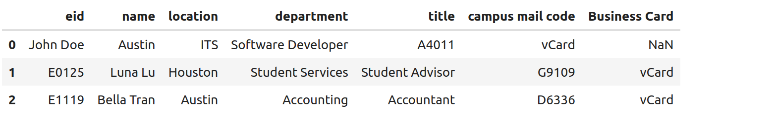
Something interesting (and not in a good way) has happened… the first row has a value
of NaN for the Business Card column and every other is off by one; for example,
it has a value of John Doe for the eid column.
A Word on Missing Values and the Nan Value
The pandas library has multiple ways of representing missing values. We’ll discuss dealing with missing
values more in the next lecture, and we will get practice working with missing values throughout the
semester. For now, know that the Nan value showing up in the above DataFrame is the numpy “Nan”
value (i.e., np.nan), and it has some interesting properties. For example, it never “equals”
any other value when testing with the == operator.
In-Class Exercise.
Read the employees_bad.csv file into a DataFrame, and select the NaN value from the 0th row.
Confirm that the NaN value from the 0th row is not
==to the numpynanvalue.Replace the
==operator in step 2 with theisoperator. What do you find?
Warning
The main takeaway at this time is that dealing with missing values is subtle and tricky. Care is required to make sure your DataFrame and the calculations you do with it aren’t corrupted in the presence of missing values.
See the pandas documentation [3] for more about missing data.
Solutions:
# import numpy
>>> import numpy as np

# read the bad csv file
>>> employees_bad = pd.read_csv('employees_bad.csv')

# grab the "Business Card" column from the 0 row
>>> r1_nan = employees_bad.iloc[[0]].get("Business Card")

# confirm it is not == to np.nan
>>> r1_nan == np.nan
False

# confirm it is not == to np.nan
>>> r1_nan is np.nan
True
Functions on DataFrames
There are a number of important functions that we will use throughout the semester. Here are a few important ones to know now:
head(): returns first 5 rows of the dataset.tail(): returns last 5 rows of the dataset.shape: returns the number of rows and columns in the dataset.info(): returns the datatype of each column in the datasetcount(): returns the number of rows of each column in the dataset.min: returns minimun value of numeric column specifiedmax:returns maximum value of numeric column specifiedunique: return unique values for given columnvalue_counts: return counts of each value for a given column
In-Class Exercise.
Create a pandas DataFrame of used cars data based on the
datasets/unit01/used_cars_data.csvfile in the class repo.Print the first 5 and last 5 rows of the data set.
How many rows and how many columns are in the dataset?
Are any columns missing data? If so, which ones? And how many rows are missing for each?
References and Additional Resources
Pandas Documentation (2.2.0). https://pandas.pydata.org/docs/index.html
Input/Output: Pandas Documentation (2.2.0). https://pandas.pydata.org/docs/reference/io.html
Working with Missing Data: Pandas Documentation (2.2.0). https://pandas.pydata.org/docs/user_guide/missing_data.html