Introduction to Data Analysis and the Numpy Package
We will begin by giving a high-level overview of the kinds of data analysis
tasks we will be performing and why they are important. We’ll also introduce
the numpy python package and work through some examples in a Jupyter notebook
to make sure we
By the end of this module, students should be able to:
Understand what data analysis is and why (at a high level) it is important.
Have a basic understanding of the different kinds of tasks we will perform and what libraries we will use for each kind of task.
(Numpy) Understand the primary differences between the
ndarrayobject fromnumpyand basic Python lists, and when to use each.(Numpy) Utilize
ndarrayobjects to perform various computations, including linear algebra calculations and statistical operations.
Data Analysis and Manipulation
In this class, as with problems in the real world, we will be working with datasets. When we introduce Machine Learning in a couple of weeks, you will see that our algorithms and workflows require data – high quality data – in order to be effective.
Data come in different shapes and sizes:
Text data, in different formats and types; for example, JSON, CSV, XML, SQL, etc.
Image data, in different formats and sizes; for example, JPG, PNG, BMP, TIFF, etc.
Audio data, in different formats and sizes; for example, M4A, MP3, MP4, WAV, FLAC, etc.
Video data, in different formats and sizes; for example, MVV, MOV, MPEG4, etc.
Additionally, sometimes different types of data are combined – for example, a set of images or audio files together with some labels in text format.
While data naturally appear in all of these formats above, most of the algorithms we will be studying work on numerical data; i.e., integer and float types. We will need to prepare the data prior to using these algorithms in order for them to be effective.
Moreover, it is typical for there to be other issues with the data. Some examples include:
(Text Data) Null or missing values: with tabular text data, some rows may not contain values for every column
(Text Data) Duplicate data: rows or columns could be duplicated.
(Text Data) Irrelevant data: some columns could be irrelevant to the process being modeled.
(Image and Video Data) The samples could be of different dimensions or different resolutions.
(Audio, Image and Video Data) Samples could be processed with different codecs and there could be noise and/or distortion on the samples.
A major aspect of the work involved in applying machine learning to real-world applications involves data preprocessing; that is, analyzing the raw data to understand what you have, and transforming it into a format that can be efficiently utilized by the learning algorithms.
Without taking the necessary steps to prepare the data, the machine learning algorithms will not be effective.
Note
“Garbage in, garbage out.” -An astute COE 379L student
Big Picture: Data Analysis Taks and the Libraries We Will Use
Data analysis consists of several different kinds of tasks. We will be using Python libraries that specialize in each task type.
Numpy and Scipy – These libraries form the foundation of all of the libraries we will use. The
numpypackage, wich we will look at first, provides an efficient multi-dimensional array object, useful for performing numeric computations across vectors and matrices. Thescipypacakge, which depends on the nd-array fromnumpy, adds a number of scientific algorithms, such as algorithms from linear algebra (e.g., matrix calculations), numerical methods (e.g., integration), FFTs, etc.Pandas – The
pandaslibrary provides an efficient Series and DataFrame class for working with column/tabular data. We will make extensive use of Pandas throughout the course for data preprocessing tasks.Matplotlib/Seaborn – These are two visualization libraries, for creating plots of various kinds. We will use these libraries extensively as well, to be able to visualize the datasets we are working with.
Scikit-Learn – This is the library we will use during the first (roughly) half of the semester, for the “classical” machine learning algorithms we will employ.
Tensorflow – This is the library we will use for neural networks and deep learning.
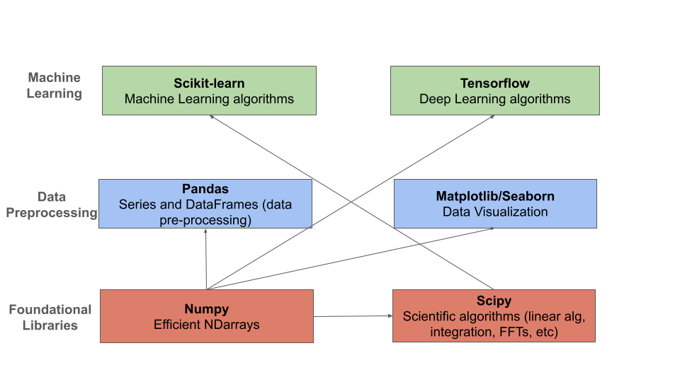
The Python libraries we will use and their relationships.
Numpy
In the remainder of this module, we will introduce the Python library numpy for working with arrays
of numerical data.
In some ways, numpy is perhaps the package we will use the least directly, but since all the
other libraries depend on its ndarray object, it will be useful to have a basic exposure to it.
We will, on occasion, use numpy functions directly on our data.
The Numpy Package
The numpy package provides a Python library for working with numerical arrays that are orders
of magnitute faster than ordinary Python lists. The primary data structure provided by numpy is the
ndarray. There are a few main reasons why working with ndarrays is faster than normal Python
lists for numerical calculations:
Storage in memory: Numpy
ndarraysare stored as continuous memory, unlike Python lists which are stored across the heap. Various algorithms can exploit this continuity to achieve significant performance gains.
2. The performance-critical blocks of numpy are written in C/C++ and are optimally compiled for
different CPU architectures.
Installing Numpy
The numpy package is available from the Python Package Index (PyPI) and can be installed on most
platforms using a Python package mananger such as pip:
[container/virtualenv]$ pip install numpy
Warning
I highly recommend you avoid installing these packages directly into the global package
namespace (i.e., executing pip install numpy directly on the VM).
Over time, you are likely to run into dependency issues and will have a hard time modifying and/or reproducing your environment in another location.
Once installed, we can import the numpy package; it is customary to import the top level package
as np, i.e.,
>>> import numpy as np
Using the Class Docker Container
We have created a Docker image available on the public Docker Hub (hub.docker.com)
Note
The class image is jstubbs/coe379l.
Use either the default (latest) tag or the :sp24 tag.
The docker image contains all of the libraries that we will need for the course, including
numpy and jupyter.
You can see a list of all of the packages installed in the poetry.lock file on the class repo. (and by the way, if you don’t know about Python Poetry, check it out!)
Numpy Arrays
The workhouse of numpy is the ndarray class. Arrays are collections of data of the same type.
Creating Arrays from lists
We can create an array in numpy from a list of integers using the np.array() function, as follows:
>>> m = np.array([1,2,3,4,5])
Numpy arrays have both a size and a shape:
>>> m.size
5

>> m.shape
(5,)
The size returns the total number of elements in the array while the shape returns the size of each
dimension of the array. The array we defined above was a 1-dimensional array (or a “1-d array”).
Numpy supports creating arrays of different dimensions. For example, we can create a 2-d or a 3-d
array by passing additional lists to the np.array() function:
# 2-d array
>>> m2 = np.array([[1,2,3,4,5], [6,7,8,9,10]])
>>> m2.size
10
>>> m2.shape
(2,5)

# 3-d array
>>> m3 = np.array([ [[1, 2], [3, 4], [5, 6]], [[-1, -2], [-3, -4], [-5, -6]]] )
>>> m3.size
12
>>> m3.shape
(2, 3, 2)
The shape of m2 is (2,5) indicating that it has 2 rows of 5 elements each.
Similarly, the shape of m3 is (2, 3, 2) because it has 2 rows,
3 columns and 2 “depth” dimensions.
Another way to think of it is this: a 2d-array is an array that has 1d-arrays as its elements. Similarly, a 3d-array is an array with 2d-arrays as its elements, etc.
Warning
Take care to note the use of open ([) and closed (]) brackets.
Ultimately, the np.array() function takes one positional argument, which
is the the list (array) of objects (elements, 1d-arrays, 2d-arrays, etc.)
If we get confused, we can always ask numpy for the dimension of an array:
>>> m3.ndim
3
Note that each row of an ndarray must have the same number of elements; the following does not work:
>>> m = np.array([[1,2,3], [6,7]])
What happens if you try the code above?
Other Functions For Creating Arrays
Numpy provides a number of other functions for creating arrays. We mention a few briefly here.
First, we can create an array of 0’s of a particular shape:
# create an array of zeros; specify the shape of the array:
>>> m = np.zeros((3,4))

# m is a 3x4 array full of 0's:
>>>  m
array([[0., 0., 0., 0.],
   [0., 0., 0., 0.],
   [0., 0., 0., 0.]])

# what are the following values?
>>> m.shape

>>> m.size

>>> m.ndim
Similarly, we can create an array of random numbers, though we will need to import the random
package from numpy. Here we create an array of random integers over a specific range:
>>> from numpy import random
# create a 3x4 array of random integers between 0 and 100
>>> m = random.randint(100, size=(3, 4))
>>> m
array([[22, 33, 35, 66],
   [41, 84, 25, 89],
   [23, 99, 94,  3]])
Note that the value of the size parameter is a tuple with the sizes of each dimension.
We can also create arrays of floating points. In this case, we pass the size as a set of integers, and the values in the array will be between 0 and 1.
# create a 3x5 array of floats between 0 and 1
>>> random.rand(3, 5)
array([[0.54639945, 0.50198887, 0.75635589, 0.29956539, 0.02611014],
   [0.08913416, 0.85613525, 0.02844888, 0.84614452, 0.95455804],
   [0.06800074, 0.04932212, 0.02175548, 0.53220075, 0.3348725 ]])
The arange() function can be used to create numpy arrays
with elements spaced evenly as defined in an interval.
It takes the following parameters:
start: starting element of array (fefault is 0).
stop: end of the interval.
step: step size of the internal (default is 1).
# create a 1D array between 0 and 10, with a step size of 2
>>> m = np.arange(start=0, stop=10, step=2)
>>> m
array([0, 2, 4, 6, 8])
As you can see the stop is given as 10, so it will not be included in the array.
Indexing and Slicing
Array indexing with numpy works the same as normal Python lists – we can index into the array
using the [index] notation:
>>> m = random.randint(100, size=(3))
>>> m
array([78, 37, 41])
>>> m[0]
78
>>> m[2]
41
>>> m[3]
IndexError: index 3 is out of bounds for axis 0 with size 3
Indexing multi-dimensional arrays also works, but now if we provide fewer indexes than the dimension of the array, the result is another array.
For example,
>>> m = random.randint(100, size=(3, 2))
>>> m
array([[75, 46],
   [13, 90],
   [34,  2]])

# slice a single value by providing 2 parameters (remember, they are 0-indexed!)
>>> m[1,1]
90
>>> m[2,1]
2
>>> m[1,2]
?

# providing fewer than 2 parameters results in a 1-d array:
>>> m[2]
array([34,  2])
We can also slice Numpy arrays. Like indexing, slicing works the same as Python lists:
>>> m = random.randint(100, size=(3))
>>> m
array([78, 37, 41])
>>> m[1:2]
array([37])
>>> m[1:]
array([37, 41])
With higher-dimensional arrays, one can slice in each dimension, from left to right.
>>> m = random.randint(100, size=(3, 2))
>>> m
array([[75, 46],
   [13, 90],
   [34,  2]])

>>> m[0:1, 0:2]
array([[75, 46]])

>>> m[1:]
array([[13, 90],
   [34,  2]])

>>> m[:, 1:]
array([[46],
   [90],
   [ 2]])
Array Functions
Numpy provides a number of functions for computing over the data in an array. We mention just a few here; for more details, consult the numpy documentation [1].
>>> m
array([[75, 46],
   [13, 90],
   [34,  2]])

# sum all elements in m
>>> m.sum()
260

# average all elements in m
>>> m.mean()
43.333333333333336

# maximum and minimum elements
>>> m.max()
90

>>> m.min()
2
Class Exercise.
Create a numpy array of first 10 odd numbers.
What is the output of following python code
np.arange(start = 9, stop = 0, step = -1)? Can you reshape it to a 3X3 matrix? (Hint: use reshape function)What will be the output of following code np.arange(20)[10:17]
Given an array
p = np.arange(20), how will you reverse it?Generate two 2X2 numpy arrays with random values up to 10, compute the sum of these two arrays.
References and Additional Resources
Numpy documentation – Numpy v1.26 manual.