Solution to Spambase Lab

Exercise 1. Getting and preparing the data.

Begin by downloading the file to your local machine:

# download zip file
$ wget https://archive.ics.uci.edu/static/public/94/spambase.zip

# unpack file
$ unzip spambase.zip

# check files
$ ls -l
-rwx------ 1 jstubbs jstubbs 702942 May 22  2023 spambase.data
-rwx------ 1 jstubbs jstubbs   6429 May 22  2023 spambase.DOCUMENTATION
-rwx------ 1 jstubbs jstubbs   3566 May 22  2023 spambase.names
-rw-rw-r-- 1 jstubbs jstubbs 125537 Feb 15 10:18 spambase.zip

$ file spambase.data
spambase.data: CSV text

$ head spambase.data
0,0.64,0.64,0,0.32,0,0,0,0,0,0,0.64,0,0,0,0.32,0,1.29,1.93,0,0.96,0,0,0,0,0,0,0,0,0,0,0,0,0,0,0,0,0,0,0,0,0,0,0,0,0,0,0,0,0,0,0.778,0,0,3.756,61,278,1
0.21,0.28,0.5,0,0.14,0.28,0.21,0.07,0,0.94,0.21,0.79,0.65,0.21,0.14,0.14,0.07,0.28,3.47,0,1.59,0,0.43,0.43,0,0,0,0,0,0,0,0,0,0,0,0,0.07,0,0,0,0,0,0,0,0,0,0,0,0,0.132,0,0.372,0.18,0.048,5.114,101,1028,1
0.06,0,0.71,0,1.23,0.19,0.19,0.12,0.64,0.25,0.38,0.45,0.12,0,1.75,0.06,0.06,1.03,1.36,0.32,0.51,0,1.16,0.06,0,0,0,0,0,0,0,0,0,0,0,0,0,0,0,0.06,0,0,0.12,0,0.06,0.06,0,0,0.01,0.143,0,0.276,0.184,0.01,9.821,485,2259,1

Note that the file has no header row. Let’s add that:

# open the file in an editor, e.g., vim, and paste the following line at the top
"word_freq_make,word_freq_address,word_fre_all,word_freq_3d,word_freq_our,word_freq_over,word_freq_remove,word_freq_internet,word_freq_order,word_freq_mail,word_freq_receive,word_freq_will,word_freq_people,word_freq_report,word_freq_addresses,word_freq_free,word_freq_business,word_freq_email,word_freq_you,word_freq_credit,word_freq_your,word_freq_font,word_freq_000,word_freq_money,word_freq_hp,word_freq_hpl,word_freq_george,word_freq_650,word_freq_lab,word_freq_labs,word_freq_telnet,word_freq_857,word_freq_data,word_freq_415,word_freq_85,word_freq_technology,word_freq_1999,word_freq_parts,word_freq_pm,word_freq_direct,word_freq_cs,word_freq_meeting,word_freq_original,word_freq_project,word_freq_re,word_freq_edu,word_freq_table,word_freq_conference,char_freq_;,char_freq_(,char_freq_[,char_freq_!,char_freq_$,char_freq_#,capital_run_length_average,capital_run_length_longest,capital_run_length_total,Class"

Now, read the file into a pandas DataFrame:

>>> import pandas as pd
>>> data = pd.read_csv("spambase.csv")

We can check and print the number of rows and columns using different methods; e.g., the info() funcion:

>>> data.info()
<class 'pandas.core.frame.DataFrame'>
RangeIndex: 4601 entries, 0 to 4600
Data columns (total 58 columns):
#   Column                      Non-Null Count  Dtype
---  ------                      --------------  -----
0   word_freq_make              4601 non-null   float64
1   word_freq_address           4601 non-null   float64
.  .  .

There are 4,601 rows and 58 columns.

Exercise 2. Data Exploration.

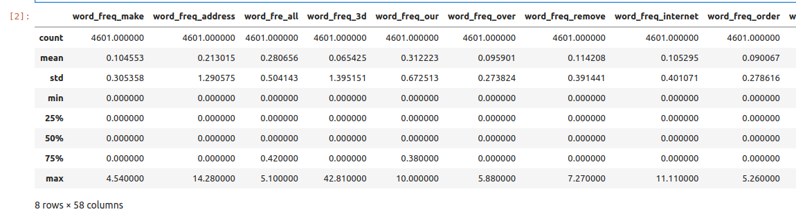
First, we compute standard statistics for each of the columns in the dataset, including: count, mean, standard deviation, min and max.

>>> data.describe()

Next, we determine if there are any duplicate rows in the data set. If there are any duplicate rows, we remove them.

# look for duplicate entries in the data
>>> data.duplicated().sum()

391

>>> data = data.drop_duplicates()

Next, we determine if there are any missing values in the dataset. There are different ways to do this. One way it to look at the output of data.info() – it shows that all columns contain 4,601 non-null rows, the number of total rows in the dataset. Alternatively, here is a one-liner that provides a True/False response:

>>> data.isnull().values.any()
False

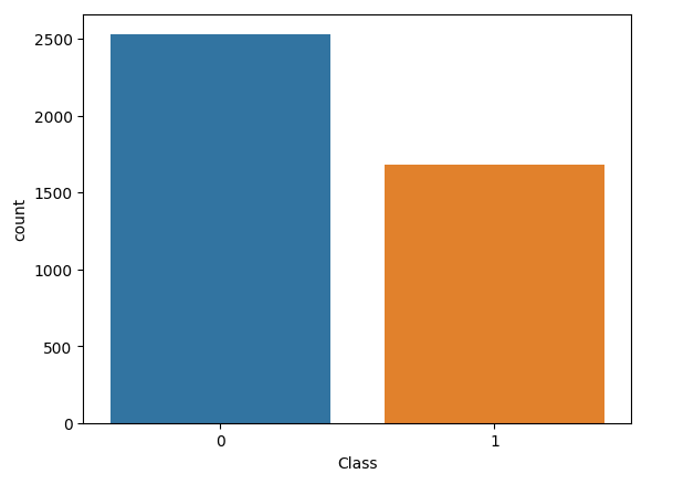
Finally, we determine how many rows are spam and how many are not spam. We know this is controlled by the Class column. Again, there are different techniques. For example, we could use a filter to check the number of values for each class label:

>>> data[data['Class'] == 0]
. . .
[2531 rows x 58 columns]

>>> data[data['Class'] == 1]
. . .
[1679 rows x 58 columns]

We see there are 2,531 non-spam and 1,679 spam rows. We could also create a count plot to visualize this:

>>> import seaborn as sns
>>> sns.countplot(data=data,x='Class')
>>> plt.show()

Exercise 3. Split and Fit.

We split the data into training and test datasets using the train_test_split() function. To make sure our split is reproducible, we use the random_state parameter, and to ensure that it maintains roughly the proportion of spam and non-spam emails we use the stratify parameter:

>>> from sklearn.model_selection import train_test_split
>>> X = data.drop('Class',axis=1)
>>> y = data['Class']
>>> X_train, X_test, y_train, y_test = train_test_split(X, y, test_size=0.3, stratify=y, random_state=1)

With the data split, we can train the model.

>>> from sklearn.linear_model import SGDClassifier
>>> clf = SGDClassifier(loss="perceptron", alpha=0.01)
>>> clf.fit(X_train, y_train)

Exercise 4. Validation and Assessment.

We evaluate our model and the test data:

>>> from sklearn.metrics import accuracy_score
>>> accuracy_test=accuracy_score(y_test, clf.predict(X_test))
>>> print('Accuracy on test data is : {:.2}'.format(accuracy_test))

Accuracy on test data is : 0.77

as well as on the training data:

>>> accuracy_train=accuracy_score(y_train, clf.predict(X_train))
>>> print('Accuracy on train data is : {:.2}'.format(accuracy_train))

Accuracy on train data is : 0.72

We plot a confusion matrix for our model:

>>> from sklearn.metrics import ConfusionMatrixDisplay
>>> cm_display = ConfusionMatrixDisplay.from_estimator(clf, X_test, y_test,
                                               cmap=plt.cm.Blues,normalize=None)

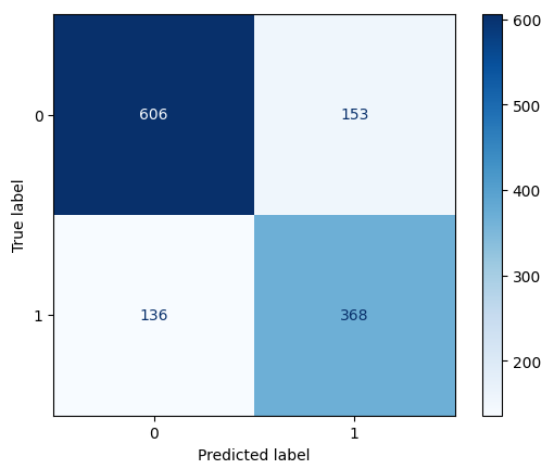
This shows that the model predicted that spam emails were non-spam 136 times and predicted that non-spam emails were spam 153 times. The model also correctly predicted 606 non-spam emails and 368 spam emails.