Hands-on Transformers
In this module, we introduce the transformers library from Hugging Face and we show some
initial examples of working with pre-trained models for solving NLP tasks.
By the end of this module, students should be able to:
Use pipeline objects to work with pre-trained models on a number of NLP tasks.
Understand the basic components of a pipeline, including data preprocessing, model application and post-processing.
Understand how to use a Tokenizer to convert text to numerical inputs and to convert numerical values back to text, including different variants on the API (returning tensors, batching, padding, etc).
Work with (pre-trained) model checkpoints from the HuggingFace Hub in various ways, including with attention heads for different NLP tasks.
Introduction to Pipelines
As we mentioned briefly in the previous module, pipeline objects from the transformers library
are basic abstractions that simplify interactions with large models. We’ll look at the steps
of a pipeline in more detail momentarily, but first let’s see some basic examples.
The simplest way to create a pipeline is to use the pipeline function and pass a specific
task type. For example, we can create a pipeline by specifying the English to French translation
task type, translation_en_to_fr:
from transformers import pipeline
en_to_fr_translator = pipeline("translation_en_to_fr")
This bit of code first looks up the default model for this task type and checks whether that model has already been downloaded to your huggingface cache directory. If not, it downloads it to the cache directory and then instantiates the model.
(Note that, by default, the huggingface cache directory is ~/.cache/huggingface, but you can
change that by setting the $HF_HOME environment variable).
We can now pass it some input and directly get some output:
en_to_fr_translator("Hello, my name is Joe.")
-> [{'translation_text': 'Bonjour, mon nom est Joe.'}]
We can pass it multiple inputs as well, as a Python list:
en_to_fr_translator(["Machine learning is a branch of Artificial Intelligence",
                 "The United States Declaration of Independence was written in 1776."])
-> [{'translation_text': 'L’apprentissage automatique est une branche de l’intelligence artificielle'},
    {'translation_text': "La Déclaration d'indépendance des États-Unis a été rédigée en 1776."}]
The transformers library includes many recognized tasks with default models. There are task types from each of the following areas:
Computer Vision, including text-to-image, image-to-text, and image-to-image tasks.
Natural Language Processing, including sentiment analysis, language translation and question answering tasks.
Audio processing, including text-to-speech, audio classification and speech recognition tasks.
Multimodal, including document question and answering (i.e., answering questions on a visual document) and visual question and answering (answering open-ended questions based on an image).
Some specific examples include:
translation_xx_to_yy– Language translation from language xx to language yy.sentiment-analysis– Also called text classification, i.e., classifying the sentiment expressed in text.summarization– Producing a summary of the input text.image-classification– Classifying objects in an image.image-to-text– Generate a summary/caption for an image.
More information is available on the HuggingFace documentation site, here ([2]). For a complete list of valid task definition strings, see the pipeline API reference.
And just as with the language translation pipeline we defined above, we can defined similar pipelines for other tasks. For example, a text summarization pipeline:
summarizer = pipeline("summarization")
summarizer("""NLP is one of the oldest areas of AI and has a long history dating back at least to the 1950s.
    One of the first efforts to garner public attention was the Georgetown-IBM experiment in 1954, which
    attempted automatically translate Russian sentences to English.
    Here is a screenshot from an early, famous NPL program called ELIZA, developed at MIT between 1964 and
    1967. THe ELIZA program prompted users with questions in natural language text and enabled them to
    submit answers, also in natural language. The goal was to simulate a psychotherapy session.""")

Output ->
[{'summary_text': " NPL is one of the oldest areas of AI and has a long history dating back at least to
  the 1950s . The Georgetown-IBM experiment in 1954 attempted to automatically translate Russian sentences
  to English . MIT's ELIZA program prompted users with questions in natural language text and enabled
  them to answer them with answers ."}]
Some tasks, however, do not have a default model. For example, if we try to build a pipeline for the English to Spanish translation task, we get an error:
en_to_es_translator = pipeline("translation_en_to_es")
-> ValueError: The task does not provide any default models for options ('en', 'es')
For these, we need to pass a specific model to use. Let’s see how we can explore the HuggingFace Hub to find such a model.
HuggingFace Hub
There are many models for English to Spanish translation available from the transformers library. How do we go about finding them? One option is to use the HuggingFace Hub to search for models by task. The transformers library can utilize any of the publicly available models on the hub.
Navigate to the HuggingFace website, here.
Click Models to browse and search for models. As of the time of this writing there are over 595,000 models on the hub.
Click to filter by task type; we would like to search for models that can perform the “Translation” task type, so we click that.
Next, select the “Languages” filter tab to filter by languages. We are interested in English to Spanish, so we select those.
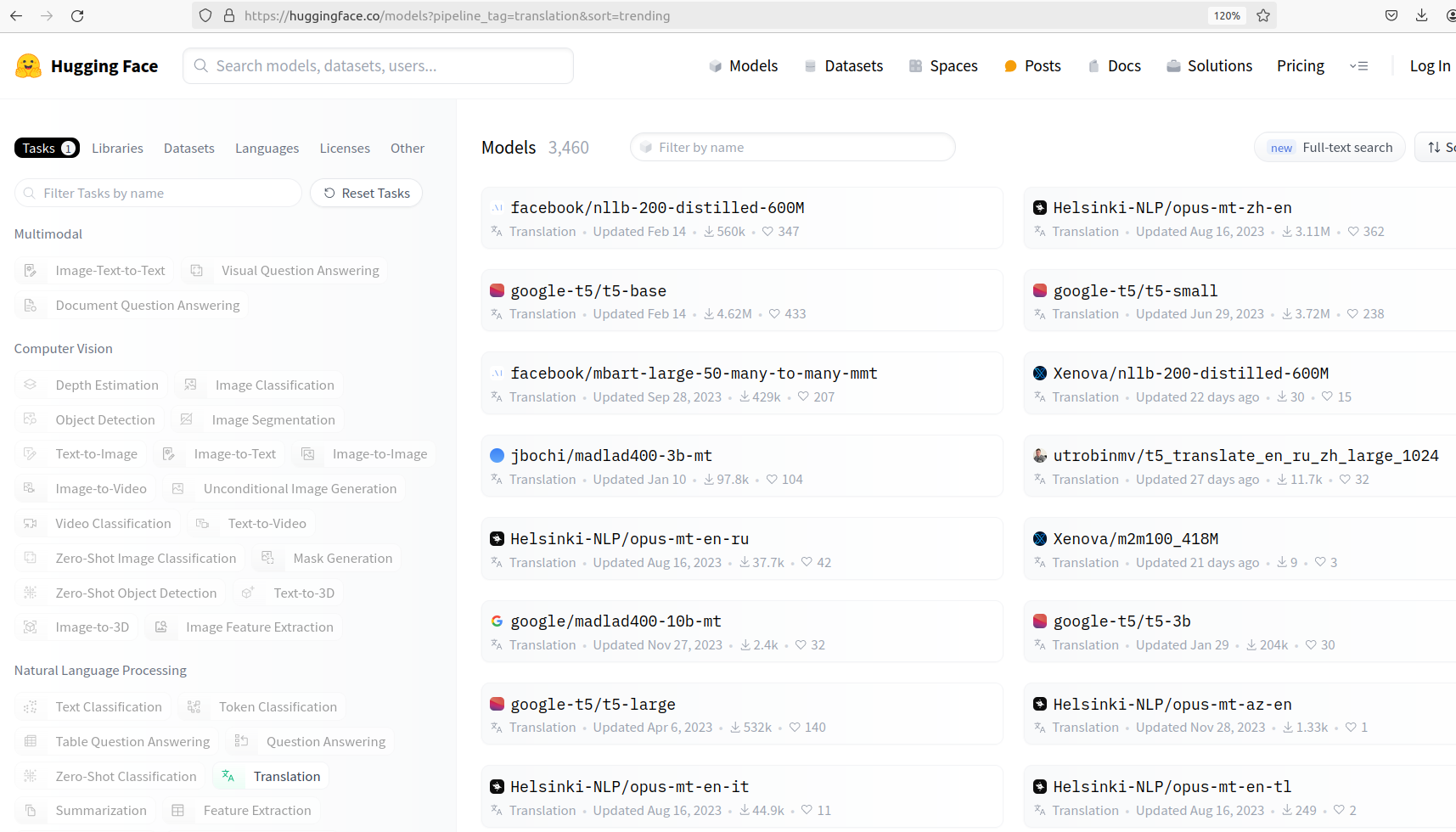
The models associated with the “Translation” task type.
This should filter the list of models down to around 157 models. We can see the task associated with each of the models (“Translation” in this case) as well as the number of downloads, and the number of hearts. By clicking a model, we can see more information about it.

Translation models that include English and Spanish.
Let’s select the Helsinki-NLP/opus-mt-es-en model. By clicking it we are taken to the main
page for the model. There we can see the model card for the model. A model card is an idea that
is gaining traction in the ML community. It is a separate file that accompanies the model and provides
additional metadata about it. On HuggingFace, model cards are always captured in markdown, contained
in a file called README.md.
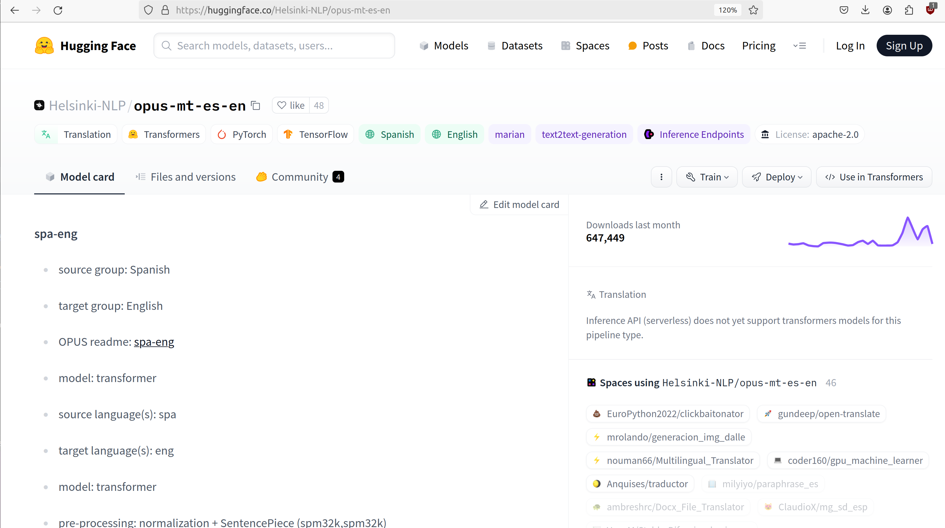
The model card for the the Helsinki-NLP/opus-mt-es-en model.
This particular model card doesn’t have a lot of information on it, but it does include the performance of this model on different benchmarks. More about benchmarks in a future lecture.
On the Files and Versions tab, we can see the actual physical files associated with the model. On
the HuggingFace Hub, models are just git repositories containing files. Note that the actual
serialized model has been made available for both pytorch and tensorflow (the pytorch_model.bin
and tf_model.h5 files, respectively). We also see the README.md file which is the model’s
model card.
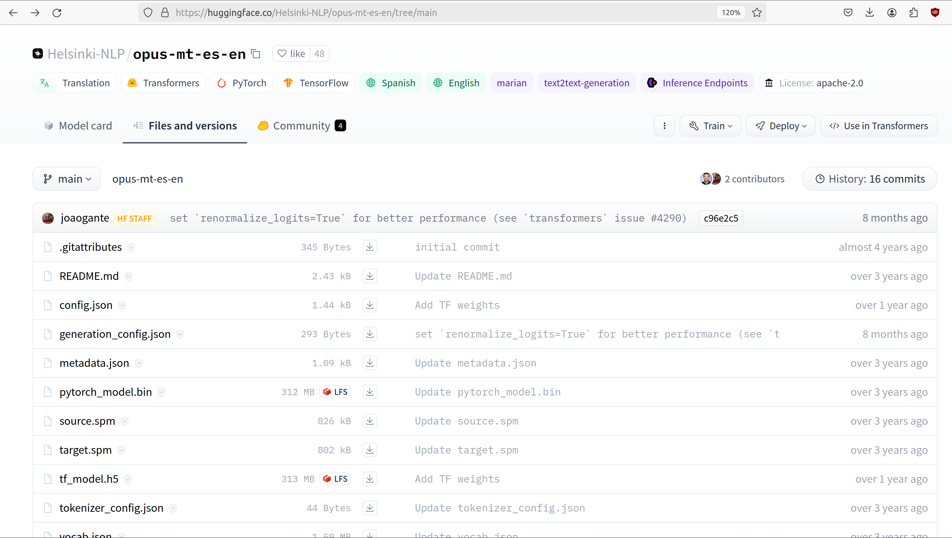
The git repository of files for the the Helsinki-NLP/opus-mt-es-en model.
Working With Model IDs
Let’s use this model in some code. We can use the same pipeline() function as before,
but this time we’ll use the model= argument to specify the model we want to use. Models on the
HuggingFace Hub have ids similar to docker container images, where a namespace indicates the user
or organization that created and owns the model. The namespace precedes the name of the model itself.
Note that, also like DockerHub, some models do not have a namespace. These are models that are
maintained by HuggingFace itself, as opposed to the community. For example,
distilbert-base-uncased is a model ID without a namespace while
google-bert/bert-base-uncased is a model ID associated with the google-bert
organization.
When there is a namespace, the namespace and the model name are separated by a / character,
as in <name_space>/<model_name> (this is the same as on the Docker Hub).
In our langauge translation model example above, Helsinki-NLP is the namespace and
opus-mt-es-en is the model name. The Helsinki-NLP namespace is owned by the
Language Technology Research Group at the University of Helsinki, see
here for more details.
en_sp_translator = pipeline(model="Helsinki-NLP/opus-mt-en-es")
en_sp_translator("Hello, my name is Joe.")
-> [{'translation_text': 'Hola, mi nombre es Joe.'}]
And we don’t need to restrict ourselves to text tasks. We can use computer vision models just
as easily with the pipeline() function. Let’s see an example of the “image-to-text” task.
# create a pipeline with the default model for the task
image_to_text = pipeline('image-to-text')

# use the model on an image; in this case we can simply pass it the path to a file
image_to_text("../data/panda.jpeg")
-> [{'generated_text': 'a large black bear sitting on top of a rock '}]
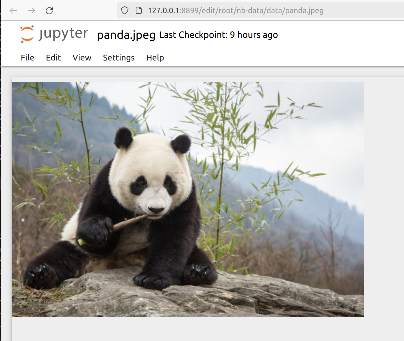
The panda.jpeg image passed to the image_to_text pipeline.
Model Architectures and Checkpoints
HuggingFace distinguishes model architectures from checkpoints; the former represents
the structure of the model (e.g., how many layers, how many trainable parameters, etc.)
while the latter includes both the architecture and the trained parameters (i.e., weights).
For example, BERT is a model architecture while google-bert/bert-base-uncased is a model
checkpoint. Note that when we say model, we usually mean a model checkpoint, but sometimes
there can be ambiguity.
Components of a Pipeline
In general, the following steps must be taken to perform inference with a model on some input text:
Convert the raw text to tokens (i.e., input ids) using a tokenizer.
Apply the model to the input ids to produce logits, that is, raw numeric values.
Post-process the outputs of the model to produce probabilities (e.g., through the application of softmax) and then class labels.
These high-level steps are depicted in the diagram below:
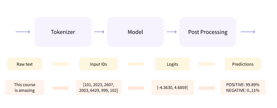
The basic components of a pipeline. (Image credit: HuggingFace NLP Course: Behind the Pipeline [1])
Each step involves multiple complexities that we will explain. We will begin with the tokenizer.
Tokenizers
As mentioned above, the tokenizer converts raw text to a series of (integer) token ids. There are various methods for implementing tokenizers. Just like any other data preprocessing method, it is critical that the exact steps used to tokenize the text for training are also used for inference. Thus, in general, we associate a specific tokenizer to each model version/checkpoint.
We’ll work with the bert-base-uncased model checkpoint to illustrate the concepts. This model is
the BERT base model introduced in the 2018 paper
BERT: Pre-training of Deep Bidirectional Transformers for Language Understanding.
You can read more about the model from its model card, here.
The transformers library provides the AutoTokenizer class to simplify loading the tokenziers
associated with a model. Specifically, the from_pretrained() method can be used to load the
tokenizer in one command:
from transformers import AutoTokenizer
checkpoint = "bert-base-uncased"
tokenizer = AutoTokenizer.from_pretrained(checkpoint)
The transformers class has instantiated a tokenizer that we can immediately use on a sentence to get a sense of how it works:
d = tokenizer("The food was good, not bad at all.")
print(d)
->
{'input_ids': [101, 1996, 2833, 2001, 2204, 1010, 2025, 2919, 2012, 2035, 1012, 102],
 'token_type_ids': [0, 0, 0, 0, 0, 0, 0, 0, 0, 0, 0, 0],
 'attention_mask': [1, 1, 1, 1, 1, 1, 1, 1, 1, 1, 1, 1]
}
A dictionary is returned with three keys; input_ids are the tokens returned for our input sentence.
We’ll discuss the other keys in a minute. We can also turn the IDs back to tokens; we use the
convert_ids_to_tokens() method to do that:
tokenizer.convert_ids_to_tokens(d['input_ids'])
->
['[CLS]',
'the',
'food',
'was',
'good',
',',
'not',
'bad',
'at',
'all',
'.',
'[SEP]']
We see that in addition to handling the words and punctuation, two “special” tokens were inserted:
the [CLS] and [SEP] tokens. If we look at the
Training Procedure
section on the model card, we see that the model was trained in part on the following task:
given two sentences, sentence A and sentence B, predict whether sentence A and B correspond to
two consecutive sentences in the original text. The model was shown a mix of both consecutive
sentences and sentences that were not consecutive as part of training. In order to structure the
input, the special [CLS] and [SEP] tokens were inserted, as follows:
[CLS] Sentence A [SEP] Sentence B [SEP]
The tokenizer allows us to mimic this procedure — we simply pass a pair of sentences as individual arguments to the tokenizer:
d2 = tokenizer("The food was good, not bad at all.", "The food was bad, not good at all.")
print(d2)
->
{'input_ids': [101, 1996, 2833, 2001, 2204, 1010, 2025, 2919, 2012, 2035, 1012, 102,
                    1996, 2833, 2001, 2919, 1010, 2025, 2204, 2012, 2035, 1012, 102],
 'token_type_ids': [0, 0, 0, 0, 0, 0, 0, 0, 0, 0, 0, 0, 1, 1, 1, 1, 1, 1, 1, 1, 1, 1, 1],
 'attention_mask': [1, 1, 1, 1, 1, 1, 1, 1, 1, 1, 1, 1, 1, 1, 1, 1, 1, 1, 1, 1, 1, 1, 1]
}
You are probably speculating that the separators have been inserted between the sentences based on those
token id’s at the beginning and end of the input_ids lists. We can confirm
it by using the convert_ids_to_tokens() function:
tokenizer.convert_ids_to_tokens(d2['inputs_ids'])
->
['[CLS]',
'the',
'food',
'was',
'good',
',',
'not',
'bad',
'at',
'all',
'.',
'[SEP]',
'the',
'food',
'was',
'bad',
',',
'not',
'good',
'at',
'all',
'.',
'[SEP]']
This explains the token_type_ids as well — the type tracks whether the token belonged to the
first sentence (value 0) or the second (value 1).
Batching Inputs
In addition to accepting two different input arguments, as in the example above, the tokenizer objects can also accept batches of inputs, provided as a single list argument. For example:
tokenizer(["The food was good, not bad at all.", "The food was bad, not good at all."])
->
{'input_ids': [[101, 1996, 2833, 2001, 2204, 1010, 2025, 2919, 2012, 2035, 1012, 102],
               [101, 1996, 2833, 2001, 2919, 1010, 2025, 2204, 2012, 2035, 1012, 102]],
 'token_type_ids': [[0, 0, 0, 0, 0, 0, 0, 0, 0, 0, 0, 0], [0, 0, 0, 0, 0, 0, 0, 0, 0, 0, 0, 0]],
 'attention_mask': [[1, 1, 1, 1, 1, 1, 1, 1, 1, 1, 1, 1], [1, 1, 1, 1, 1, 1, 1, 1, 1, 1, 1, 1]]}
Notice how, in this case, the token_type_ids all have value 0. That is because fundamentally we are using
a different API when we pass a single Python list argument: we are using the batch API.
Returning Tensors
The input_ids object is very close to the type of object that can be fed directly into the
model, but we need to make two small changes to it first; those are:
We need to return tensor objects, in one of the supported deep learning frameworks, such as Pytorch or TensorFlow.
We need to pad the list of
input_idswith an extra dimension, because the model object presents a batch API, just like with keras and sklearn.
We can accomplish both of these by using the return_tensors argument, passing a string representing
the framework we want returned, with "pt" for Pytorch and "tf" for TensorFlow.
d = tokenizer("The food was good, not bad at all", return_tensors="pt")
tensors = d['input_ids']
print(type(tensors), tensors.shape)
print(tensors)
-> <class 'torch.Tensor'> torch.Size([1, 12])
-> tensor([[ 101, 1996, 2833, 2001, 2204, 1010, 2025, 2919, 2012, 2035, 1012,  102]])
Note the 2-dimensions, both in the shape and the output of the tensors object itself —
there are double open and closed brackets (i.e., [[ and ]]).
Returning Tensors from the Batch API and Using Padding
Just as in the example above, we can ask for tensors to be returned when using the batch API of the
tokenizer via the same return_tensors parameter. However, we have to be careful; if the inputs are
different sizes, we can run into issues. Let’s look at the following example:
tokenizer(["The food was good", "The food was bad, not good at all."], return_tensors='pt')
If we try to execute the code above, we get the following exception:
-> ValueError: Unable to create tensor, you should probably activate truncation and/or padding...
The issue is that our transformer model, like all ANNs, require rectangular inputs, but since the inputs are different length, we get an issue trying to convert to a (rectangular) tensor.
We can get around this problem by passing padding=True; e.g.,
tokenizer(["The food was good", "The food was bad, not good at all."], return_tensors='pt', padding=True)
->
{'input_ids': tensor([[ 101, 1996, 2833, 2001, 2204,  102,    0,    0,    0,    0,    0,    0],
                      [ 101, 1996, 2833, 2001, 2919, 1010, 2025, 2204, 2012, 2035, 1012,  102]]),
 'token_type_ids': tensor([[0, 0, 0, 0, 0, 0, 0, 0, 0, 0, 0, 0],
                           [0, 0, 0, 0, 0, 0, 0, 0, 0, 0, 0, 0]]),
 'attention_mask': tensor([[1, 1, 1, 1, 1, 1, 0, 0, 0, 0, 0, 0],
                           [1, 1, 1, 1, 1, 1, 1, 1, 1, 1, 1, 1]])}
What’s happened here is that transformers has adding padding, i.e., a special token, to the first, shorter
input to make it have the same length as the second input — note the 0s at the end of the first tensor in the
input_ids object. We can also see the actual tokens used
d3 = tokenizer(["The food was good", "The food was bad, not good at all."], padding=True)
tokenizer.convert_ids_to_tokens(d3['input_ids'][0])
->
['[CLS]',
'the',
'food',
'was',
'good',
'[SEP]',
'[PAD]',
'[PAD]',
'[PAD]',
'[PAD]',
'[PAD]',
'[PAD]']
Finally, this also explains the last object returned, the attention_mask. This object encodes which
elements of the input_ids vector should be ignored (or “masked”) when fed through the network. We do not
want the padding tokens to be interpreted as part of the original input data so we mask them from the model.
If we look back at the output above, we see the mask has a 0 in each of the elements where the original input vector had a padding token.
{'input_ids': tensor([[ 101, 1996, 2833, 2001, 2204,  102,    0,    0,    0,    0,    0,    0],
                      [ 101, 1996, 2833, 2001, 2919, 1010, 2025, 2204, 2012, 2035, 1012,  102]]),
'attention_mask': tensor([[1, 1, 1, 1, 1, 1, 0, 0, 0, 0, 0, 0],
                          [1, 1, 1, 1, 1, 1, 1, 1, 1, 1, 1, 1]])}
Models from Checkpoints and Language Embeddings
The tensors we computed in the previous section can be fed directly into the model associated with
the original checkpoint. We use the AutoModel class and the from_pretrained() method,
analogous to how we instantiated the tokenizer:
from transformers import AutoModel
model = AutoModel.from_pretrained(checkpoint)

model(tensors)
We get a BaseModelOutput object which includes a large set of tensors.
BaseModelOutputWithPoolingAndCrossAttentions(last_hidden_state=tensor([[[-0.0231, -0.0906, -0.2436,  ..., -0.1892,  0.3635,  0.2982],
        [-0.2885, -0.8670, -0.8317,  ..., -0.1848,  0.9399,  0.2939],
        [ 0.0991, -0.4587,  0.3661,  ..., -0.0423, -0.0259,  0.0489],
        ...,
        [-1.2494, -0.4512, -0.0637,  ...,  0.2568,  0.7048, -0.2646],
        [ 0.5333,  0.0407, -0.4287,  ...,  0.4020, -0.3481, -0.4612],
        [ 0.5275,  0.2445,  0.0053,  ...,  0.3517, -0.5527, -0.3193]]],
    grad_fn=<NativeLayerNormBackward0>), pooler_output=tensor([[-8.9383e-01, -4.4092e-01, -9.1071e-01,  7.6117e-01,  6.6928e-01,
        -4.6003e-02,  9.2318e-01,  2.5568e-01, -8.2578e-01, -9.9998e-01,
. . .
We can also apply the embeddings.word_embeddings() method of the model directly to our
tokens to see the language embeddings:
print(model.embeddings.word_embeddings(tensors))
->
tensor([[[ 0.0136, -0.0265, -0.0235,  ...,  0.0087,  0.0071,  0.0151],
     [-0.0446,  0.0061, -0.0022,  ..., -0.0363, -0.0004, -0.0306],
     [-0.0179, -0.0035, -0.0022,  ..., -0.0005,  0.0112, -0.0379],
     ...,
     [-0.0546,  0.0065, -0.0213,  ...,  0.0427,  0.0057, -0.0381],
     [-0.0207, -0.0020, -0.0118,  ...,  0.0128,  0.0200,  0.0259],
     [-0.0145, -0.0100,  0.0060,  ..., -0.0250,  0.0046, -0.0015]]],
   grad_fn=<EmbeddingBackward0>)
At this point we have performed the first two steps of the inference process. We need to post-process the output, and for that we need to discuss different model heads.
Model Heads and Post-processing
When we used AutoModel.from_pretrained(), we loaded the base model which produces, for each input, an output
vector of relatively high dimension, called the hidden states or the features for the input. We can think
of this output as the associated “features” of the input, computed from the model’s “understanding” of the
structure of language.
But we cannot use these features directly in any NLP task. For that, we need to supply an extra layer to the model, called a head, for the specific task we are interested in. The inputs to the head will be the outputs of the base model, i.e., the output of the last hidden layer.
We can get the shape out the output using the last_hidden_state attribute of an output, like so:
inputs = tokenizer("The food was good, not bad at all.", return_tensors="pt")['input_ids']
output = model(inputs)
output.last_hidden_state.shape
-> torch.Size([1, 12, 768])
The dimensions returned are as follows:
batch size – how many inputs were processed at a time; (in our case, 1 sentence).
sequence length – the length of the numerical representation of the sequence.
hidden size – the vector dimension of the hidden state.
Instead of using the AutoModel class to load the base model, we can use a different class to load a model
checkpoint with a specific task head.
For example, we can use the AutoModelForSequenceClassification class to load the same BERT model
checkpoint but with a classification task head added.
from transformers import AutoModelForSequenceClassification
model = AutoModelForSequenceClassification.from_pretrained(checkpoint)
If we run the code above, we get a warning:
Some weights of BertForSequenceClassification were not initialized from the model checkpoint at
bert-base-uncased and are newly initialized: ['classifier.bias', 'classifier.weight'].
You should probably TRAIN this model on a down-stream task to be able to use it for predictions and inference.
This warning is telling us that our base checkpoint did not include such a task head, so transformers initialized a random one. Thus, we should not expect good performance from this model. Instead we should fine-tune the model using a labeled dataset. We’ll look at that next time.
Instead, let’s load a different checkpoint from the HuggingFace Hub, one that has already been fine-tuned with
a classification head. We’ll use the distilbert-base-uncased-finetuned-sst-2-english checkpoint; you
can read more about it
here.
checkpoint = "distilbert-base-uncased-finetuned-sst-2-english"
model2 = AutoModelForSequenceClassification.from_pretrained(checkpoint)
outputs = model(inputs2)
outputs
-> SequenceClassifierOutput(loss=None, logits=tensor([[-0.0956, -0.0271]], grad_fn=<AddmmBackward0>),
    hidden_states=None, attentions=None)
We see that the output is now a SequenceClassifierOutput, which has a logits attribute with a shape:
outputs.logits.shape
-> torch.Size([1, 2])

outputs.logits
-> tensor([[-3.9782,  4.3248]], grad_fn=<AddmmBackward0>)
Note that these are not probabilities but the raw outputs from the model; to convert them to probabilities, we need to normalize them with the softmax function. We can use the pytorch or tensorflow. Below we use pytorch since we had previously asked for pytorch tensors:
import torch
predictions = torch.nn.functional.softmax(outputs2.logits, dim=-1)
print(predictions)
-> tensor([[2.4772e-04, 9.9975e-01]], grad_fn=<SoftmaxBackward0>)
These are the probabilities of the labels the model is predicting for our sentence. We can use the model’s
config.id2label attribute to see the labels it is using:
model.config.id2label
-> {0: 'NEGATIVE', 1: 'POSITIVE'}
Thus, we see that the model has classified the sentence as positive with 99.97% confidence. We can wrap this up into a simple post-processing function that is batch-ready, as follows:
def get_prediction(logits):
    results = []
    predictions = torch.nn.functional.softmax(outputs2.logits, dim=-1)
    for p in range(len(predictions)):
        if predictions[p][0] > predictions[p][1]:
            results.append(model.config.id2label[0])
        else:
            results.append(model.config.id2label[1])
    return results
Exercise. Let’s bring everything together in a single coding exercise. The goal here is to call the entire, end-to-end process on a set of inputs. We’ll break it down into a series of 5 steps. Try coding up the following:
Create a Python list of 5 or 6 input sentences to try the model on.
Tokenize the inputs, making sure to generate tensors that can be passed to the model. (Hint: which API are you using from the tokenizer? Do you need to do anything special to get input_ids that can be passed to the model?)
Pass the tokens output in step 2 to the model to get the raw logits.
Pass the logits returned from the model in step 3 to our post-processing function, defined above, to produce the predictions for each sentence.
Display the predictions.
Solution. Here is a solution.
# a list of inputs to try our model on
inputs = ["I am happy", "I am sad", "This is good", "This is bad", "I enjoyed the pizza", "I am worried about the exam"]

# tokenize the inputs; we'll need to use padding here, and we'll just grab the input_ids object
tokens = tokenizer(inputs, return_tensors="pt", padding=True)['input_ids']

# pass the tokens through the model
outputs = model(tokens)

# get predictions from our model outputs using the post-processing function
predictions = get_prediction(outputs.logits)

# print the prediction
for i in range(len(inputs)):
    print(f"Sentence: {inputs[i]}; prediction: {predictions[i]};
Additional References
HuggingFace NLP Course. Chapter 2: Behind the Pipeline. https://huggingface.co/learn/nlp-course/chapter2/2
HuggingFace Tasks. https://huggingface.co/tasks